Ampere's Law
The 4th Maxwell's Equation
On this page, we'll explain the meaning of the last of Maxwell's Equations, Ampere's Law, which is given in Equation [1]:
Ampere was a scientist experimenting with forces on wires carrying electric current. He was doing these experiments back in the 1820s, about the same time that Farday was working on Faraday's Law. Ampere and Farday didn't know that there work would be unified by Maxwell himself, about 4 decades later. Forces on wires aren't particularly interesting to me, as I've never had occassion to use the very complicated equations in the course of my work (which includes a Ph.D., some stints at a national lab, along with employment in the both defense and the consumer electronics industries). So, I'm going to start by presenting Ampere's Law, which relates a electric current flowing and a magnetic field wrapping around it:
Equation [2] can be explained: Suppose you have a conductor (wire) carrying a current, I. Then this current produces a Magnetic Field which circles the wire.
The left side of Equation [2] means: If you take any imaginary
path that encircles the wire,
and you add up the Magnetic Field at each point along that path, then it
will numerically equal the amount of current that is encircled by
this path (which is why we write Let's do an example for fun. Suppose we have a long wire carrying a constant electric current, I [Amps]. What is the magnetic field around the wire, for any distance r [meters] from the wire? Let's look at the diagram in Figure 1. We have a long wire carrying a current of I Amps. We want to know what the Magnetic Field is at a distance r from the wire. So we draw an imaginary path around the wire, which is the dotted blue line on the right in Figure 1: 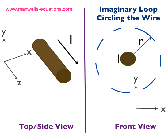 Figure 1. Calculating the Magnetic Field Due to the Current Via Ampere's Law. Ampere's Law [Equation 2] states that if we add up (integrate) the Magnetic Field along this blue path, then numerically this should be equal to the enclosed current I.
Now, due to symmetry, the magnetic field will be uniform (not varying) at
a distance r from the wire. The path length of the blue path
in Figure 1 is equal to the circumference of a circle of radius r:
If we are adding up a constant value for the magnetic field (we'll call it H), then the left side of Equation [2] becomes simple:
Hence, we have figured out what the magnitude of the H field is. And since r was arbitrary, we know what the H-field is everywhere. Equation [3] states that the Magnetic Field decreases in magnitude as you move farther from the wire (due to the 1/r term). So we've used Ampere's Law (Equation [2]) to find the magnitude of the Magnetic Field around a wire. However, the H field is a Vector Field, which means at every location is has both a magnitude and a direction. The direction of the H-field is everywhere tangential to the imaginary loops, as shown in Figure 2. The right hand rule determines the sense of direction of the magnetic field:  Figure 2. The Magnitude and Direction of the Magnetic Field Around a Wire. Manipulating the Math for Ampere's LawWe are going to do the same trick with Stoke's Theorem that we did when looking at Faraday's Law. We can rewrite Ampere's Law in Equation [2]:
On the right side equality in Equation [4], we have used Stokes' Theorem to change a line integral around a closed loop into the curl of the same field through the surface enclosed by the loop (S).
We can also rewrite the total current (
So now we have the original Ampere's Law (Equation [2]) rewritten in terms of surface integrals (Equations [4] and [5]). Hence, we can substitute them together and get a new form for Ampere's Law:
Now, we have a new form of Ampere's Law: the curl of the magnetic field is equal to the Electric Current Density. If you are an astute learner, you may notice that Equation [6] is not the final form, which is written in Equation [1]. There is a problem with Equation [6], but it wasn't until the 1860s that James Clerk Maxwell figured out the problem, and unified electromagnetics with Maxwell's Equations.
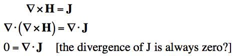
Displacement Current DensityAmpere's Law was written as in Equation [6] up until Maxwell. So let's look at what is wrong with it. First, I have to throw out another vector identity - the divergence of the curl of any vector field is always zero:
So let's take the divergence of Ampere's Law as written in Equation [6]:
So Equation [8] follows from Equations [6] and [7]. But it says that the divergence of the current density J is always zero. Is this true? If the divergence of J is always zero, this means that the electric current flowing into any region is always equal to the electric current flowing out of the region (no divergence). This seems somewhat reasonable, as electric current in circuits flows in a loop. But let's look what happens if we put a capacitor in the circuit:
 Figure 3. A Voltage Applied to A Capacitor. Now, we know from electric circuit theory that if the voltage is not constant (for example, any periodic wave, such as the 60 Hz voltage that comes out of your power outlets) then current will flow through the capacitor. That is, we have I not equal to zero in Figure 3. However, a capacitor is basically two parallel conductive plates separated by air. Hence, there is no conductive path for the current to flow through. This means that no electric current can flow through the air of the capacitor. This is a problem if we think about Equation [8]. To show it more clearly, let's take a volume that goes through the capacitor, and see if the divergence of J is zero: 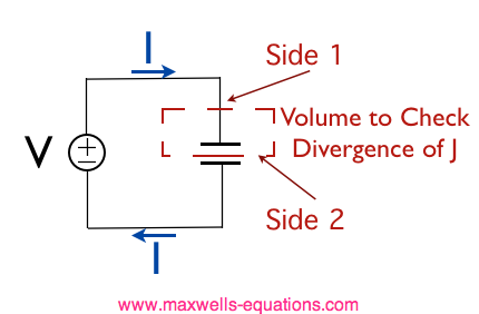 Figure 4. The Divergence of J is not Zero. In Figure 4, we have drawn an imaginary volume in red, and we want to check if the divergence of the current density is zero. The volume we've chosen, has one end (labeled side 1) where the current enters the volume via the black wire. The other end of our volume (labeled side 2) splits the capacitor in half. We know that the current flows in the loop. So current enters through Side 1 of our red volume. However, there is no electric current that exits side 2. No current flows within the air of the capacitor. This means that current enters the volume, but nothing leaves it - so the divergence of J is not zero. We have just violated our Equation [8], which means the theory does not hold. And this was the state of things, until our friend Maxwell came along. Maxwell knew that the Electric Field (and Electric Flux Density (D) was changing within the capacitor. And he knew that a time-varying magnetic field gave rise to a solenoidal Electric Field (i.e. this is Farday's Law - the curl of E equals the time derivative of B). So, why is not that a time varying D field would give rise to a solenoidal H field (i.e. gives rise to the curl of H). The universe loves symmetry, so why not introduce this term? And so Maxwell did, and he called this term the displacement current density:
This term would "fix" the circuit problem we have in Figure 4, and would make Farday's Law and Ampere's Law more symmetric. This was Maxwell's great contribution. And you might think it is a weak contribution. But the existance of this term unified the equations and led to understanding the propagation of electromagnetic waves, and the proof that all waves travel at the same speed (the speed of light)! And it was this unification of the equations that Maxwell presented, that led the collective set to be known as Maxwell's Equations. So, if we add the displacement current to Ampere's Law as written in Equation [6], then we have the final form of Ampere's Law:
And that is how Ampere's Law came into existance! Intrepretation of Ampere's LawSo what does Equation [10] mean? The following are consequences of this law:
Ampere's Law with the contribution of Maxwell nailed down the basis for Electromagnetics as we currently understand it. And so we know that a time varying D gives rise to an H field, but from Farday's Law we know that a varying H field gives rise to an E field.... and so on and so forth and the electromagnetic waves propagate - and that's cool.
This page on Ampere's Law For Circuits or whatever is copyrighted, particularly as it relates to Maxwells Equations. Copyright www.maxwells-equations.com, 2012.
|

 for encircled or enclosed current).
 .
.